Chapter 5 Common families of distributions

5.1 Exponential families

A family of pdfs (or pmfs) indexed by a parameter \(\boldsymbol{\theta}\) is called a \(k\)-parameter exponential family if it can be expressed as

\[ f\left(x|\boldsymbol{\theta}\right)=h\left(x\right)c\left(\boldsymbol{\theta}\right)\exp\left\{ \sum_{j=1}^{k}\omega_{j}\left(\boldsymbol{\theta}\right)t_{j}\left(x\right)\right\} \]

where \(h\left(x\right)\geq 0\), \(c\left(\boldsymbol{\theta}\right)\geq 0\), and \(\left\{t_{j}\left(x\right)\right\}_{j=1}^{k}\) are real-valued functions of \(x\), and where \(\left\{\omega_{j}\left(\boldsymbol{\theta}\right)\right\}_{j=1}^{k}\) are real-valued functions of the possibly vector-valued parameter \(\boldsymbol{\theta}\). I.e., \(f\left(x|\boldsymbol{\theta}\right)\) can be expressed in three parts:

• a part that depends only on the random variable(s)
• a part that depends only on the parameter(s)
• a part that depends on both the random variable(s) and the parameter(s).

Most of the parametric models you may have studied are exponential families, e.g., normal, gamma, beta, binomial, negative binomial, Poisson, and multinomial. The uniform distribution is not an exponential family (see Example 5.4 below).

Example 5.1 (Binomial random variables) Let \(X\sim\mathcal{B}\left(n,p\right)\), where \(n\) is known and \(p\in\left(0,1\right)\). Recall that \(X\) represents the number of successes in \(n\) i.i.d. Bernoulli trials and its pmf is given by

\[ f\left(x|p\right) =\binom{n}{x}p^{x}\left(1-p\right)^{n-x} \]

for \(x=0,1,\ldots,n\) and \(f\left(x|p\right)=0\) otherwise. We can write \(f\) as

\[\begin{align*} f\left(x|p\right) & = \binom{n}{x}p^{x}\left(1-p\right)^{n-x} \\ & = \binom{n}{x}p^{x}\left(1-p\right)^{n}\left(1-p\right)^{-x} \\ & = \binom{n}{x}\left(1-p\right)^{n}\left(\frac{p^{x}}{\left(1-p\right)^{x}}\right) \\ & = \binom{n}{x}\left(1-p\right)^{n}\left(\frac{p}{1-p}\right)^{x} \\ & = \binom{n}{x}\left(1-p\right)^{n}\exp\left\{ \log\left(\frac{p}{1-p}\right)^{x}\right\} \\ & = \binom{n}{x}\left(1-p\right)^{n}\exp\left\{ x\log\frac{p}{1-p}\right\}. \end{align*}\]

Now, \(n\) is known, so the only parameter is \(p\). Thus, we see that the binomial distribution is an exponential family, with

\[ h\left(x\right)=\binom{n}{x},\quad c\left(p\right)=\left(1-p\right)^{n},\quad t\left(x\right)=x,\quad\ \omega\left(p\right)=\log\frac{p}{1-p}. \]

Observe that when \(n=1\), \(X\) is a Bernoulli random variable, so it follows that the Bernoulli distribution is also an exponential family.

Example 5.2 (Poisson random variables) Let \(X\sim\text{Poisson}\left(\lambda\right)\), where \(\lambda>0\). Recall that \(X\) represents the frequency with which a specified event occurs given some fixed dimension, such as space or time, and its pmf is given by

\[ f\left(x|\lambda\right)=\frac{\mathrm{e}^{-\lambda}\lambda^{x}}{x!} \]

for \(x=0,1,2,\ldots\) and \(f\left(x|\lambda\right)=0\) otherwise. We can write \(f\) as

\[ f\left(x|\lambda\right) =\frac{\mathrm{e}^{-\lambda}\lambda^{x}}{x!} =\frac{1}{x!}\mathrm{e}^{-\lambda}\exp\left\{ \log\left(\lambda^{x}\right)\right\} =\frac{1}{x!}\mathrm{e}^{-\lambda}\exp\left\{ x\log\lambda\right\}. \]

It follows that the Poisson distribution is an exponential family, with

\[ h\left(x\right)=\frac{1}{x!},\quad c\left(\lambda\right)=\mathrm{e}^{-\lambda},\quad t\left(x\right)=x,\quad \omega\left(\lambda\right)=\log\lambda. \]

Example 5.3 (Normal random variables) Let \(X\sim\mathcal{N}\left(\mu,\sigma^{2}\right)\), where \(\mu\in\mathbb{R}\) and \(\sigma^{2}>0\). A pdf for \(X\) is given by

\[ f\left(x|\mu,\sigma^{2}\right)=\frac{1}{\sqrt{2\pi\sigma^{2}}}\exp\left\{ -\frac{\left(x-\mu\right)^{2}}{2\sigma^{2}}\right\} \]

for \(x\in\mathbb{R}\). We begin with the case that \(\sigma^{2}\) is known, so that \(\theta=\mu\). We can write \(f\) as

\[ \begin{align*} f\left(x|\mu\right) & =\frac{1}{\sqrt{2\pi\sigma^{2}}}\exp\left\{ -\frac{x^{2}-2\mu x+\mu^{2}}{2\sigma^{2}}\right\} \\ & =\frac{1}{\sqrt{2\pi\sigma^{2}}}\exp\left\{ -\frac{x^{2}}{2\sigma^{2}}\right\} \exp\left\{ -\frac{\mu^{2}}{2\sigma^{2}}\right\} \exp\left\{ x\frac{\mu}{\sigma^{2}}\right\}, \end{align*} \]

so that

\[ h\left(x\right)=\frac{1}{\sqrt{2\pi\sigma^{2}}}\exp\left\{-\frac{x^{2}}{2\sigma^{2}}\right\},\quad c\left(\mu\right)=\exp\left\{-\frac{\mu^{2}}{2\sigma^{2}}\right\},\quad t\left(x\right)=x,\quad \omega\left(\mu\right)=\frac{\mu}{\sigma^{2}}, \]

hence the normal distribution with known variance is an exponential family. Now suppose that \(\sigma^{2}\) is unknown, so that \(\boldsymbol{\theta}=\left(\mu,\sigma^{2}\right)\). We can write \(f\) as

\[ \begin{align*} f\left(x|\mu,\sigma^{2}\right) & =\frac{1}{\sqrt{2\pi\sigma^{2}}}\exp\left\{ -\frac{\left(x-\mu\right)^{2}}{2\sigma^{2}}\right\} \\ & =\frac{1}{\sqrt{2\pi}}\left(\sigma^{2}\right)^{-1/2}\exp\left\{ -\frac{x^{2}-2\mu x+\mu^{2}}{2\sigma^{2}}\right\} \\ & =\frac{1}{\sqrt{2\pi}}\exp\left\{ \log\left(\sigma^{2}\right)^{-1/2}\right\} \exp\left\{ -\frac{x^{2}}{2\sigma^{2}}+\frac{\mu x}{\sigma^{2}}\right\} \exp\left\{ -\frac{\mu^{2}}{2\sigma^{2}}\right\} \\ & =\frac{1}{\sqrt{2\pi}}\exp\left\{ -\frac{1}{2}\left(\frac{\mu^{2}}{\sigma^{2}}+\log\sigma^{2}\right)\right\} \exp\left\{ -\frac{x^{2}}{2\sigma^{2}}+\frac{\mu x}{\sigma^{2}}\right\}, \end{align*} \]

so that

\[ \begin{align*} h\left(x\right) &= \frac{1}{\sqrt{2\pi}}, & c\left(\boldsymbol{\theta}\right) &= \exp\left\{-\frac{1}{2}\left(\frac{\mu^{2}}{\sigma^{2}}+\log\sigma^{2}\right)\right\}, \\ t_{1}\left(x\right) &= -\frac{x^{2}}{2}, & \omega_{1}\left(\boldsymbol{\theta}\right) &= \frac{1}{\sigma^{2}}, \\ t_{2}\left(x\right) &= x, & \omega_{2}\left(\boldsymbol{\theta}\right) &=\frac{\mu}{\sigma^{2}}. \end{align*} \]

Thus, the normal distribution with unknown variance is also an exponential family (and the first exponential family we have seen where \(k>1\)).

Definition 5.1 The indicator function of a set \(\mathcal{A}\), denoted by \(I_{\mathcal{A}}\left(x\right)\), is the function

\[ I_{\mathcal{A}}\left(x\right)= \begin{cases} 1, & x\in \mathcal{A}\\ 0, & x\notin \mathcal{A} \end{cases}. \]

Example 5.4 (Uniform random variables) Let \(X\sim\mathcal{U}\left(a,b\right)\), where \(-\infty<a<b<\infty\). A pdf for \(X\) is given by

\[ f\left(x|a,b\right)=\frac{1}{b-a} \]

for \(x\in\left[a,b\right]\) and \(f\left(x|a,b\right)=0\) otherwise. Let \(\mathcal{A}=\left\{ x:x\in\left[a,b\right]\right\}\) and let \(I_{\mathcal{A}}\) be the indicator function of \(\mathcal{A}\). Then, we can write \(f\) as

\[ f\left(x|a,b\right)= \frac{1}{b-a}I_{\mathcal{A}}\left(x\right)= \frac{1}{b-a}I_{\left[a,b\right]}\left(x\right). \]

Notice that \(I_{\left[a,b\right]}\left(x\right)\) is not a function of \(x\) exclusively, not a function of \(\boldsymbol{\theta}=\left(a,b\right)\) exclusively, and cannot be written as an exponential. Because the entire pdf must be incorporated into \(h\left(x\right)\), \(c\left(\boldsymbol{\theta}\right)\), \(t_{j}\left(x\right)\), and \(\omega_{j}\left(\boldsymbol{\theta}\right)\), it follows that the uniform distribution is not an exponential family.

Example 5.5 (Three-parameter exponential family distribution) Consider the family of distributions with densities

\[ f\left(x|\theta\right) =\frac{2}{\Gamma\left(1/4\right)}\exp\left[-\left(x-\theta\right)^{4}\right] \]

for \(x\in\mathbb{R}\). Express \(f\left(x|\theta\right)\) in exponential family form.

Recall that the binomial theorem states that

\[ \left(x+y\right)^{n}=\sum_{k=0}^{n}\binom{n}{k}x^{k}y^{n-k}, \]

so we have

\[\begin{align*} f\left(x|\theta\right) & =\frac{2}{\Gamma\left(1/4\right)}\exp\left[-\left(x-\theta\right)^{4}\right] \\ & =\frac{2}{\Gamma\left(1/4\right)}\exp\left\{ -\sum_{k=0}^{4}\binom{4}{k}x^{k}\left(-\theta\right)^{4-k}\right\} \\ & =\frac{2}{\Gamma\left(1/4\right)}\exp\left\{ -\left[1\cdot1\cdot\theta^{4}-4x\theta^{3}+6x^{2}\theta^{2}-4x^{3}\theta+1\cdot x^{4}\cdot1\right]\right\}, \end{align*}\]

so that

\[ \begin{align*} h\left(x\right) & = \frac{2}{\Gamma\left(1/4\right)}\exp\left\{-x^{4}\right\}, & c\left(\theta\right) & = \exp\left\{-\theta^{4}\right\}, \\ t_{1}\left(x\right) & = 4x^{3}, & \omega_{1}\left(\theta\right) & = \theta, \\ t_{2}\left(x\right) & = -6x^{2}, & \omega_{2}\left(\theta\right) & = \theta^{2}, \\ t_{3}\left(x\right) & = 4x, & \omega_{3}\left(\theta\right) & = \theta^{3}. \end{align*} \]

Thus, this family of distributions is a 3-parameter exponential family.

Theorem 5.1 Random samples from \(k\)-parameter exponential families have joint distributions which are \(k\)-parameter exponential families.

Proof. Suppose that a random variable \(X\) has a pdf \(f\left(x|\theta\right)\), and that \(f\) is part of an exponential family, so that \(f\) can be written as

\[ f=h\left(x\right)c\left(\theta\right)\exp\left\{ \sum_{j=1}^{k}t_{j}\left(x\right)\omega_{j}\left(\theta\right)\right\} . \]

Now suppose that \(X_{1},X_{2},\ldots,X_{n}\) is a random sample from a population having the distribution of \(X\). It follows that the \(X_{i}\text{'s}\) are independent and identically distributed, and that each \(X_{i}\) has the same cdf as \(X\), and therefore that \(f\left(x|\theta\right)\) is a pdf for each \(X_{i}\). Then, the joint pdf of the \(X_{i}\text{'s}\) is given by

\[\begin{align*} f\left(\mathbf{x}|\theta\right) & =\prod_{i=1}^{n}f\left(x_{i}|\theta\right) \\ & =\prod_{i=1}^{n}\left[h\left(x_{i}\right)c\left(\theta\right)\exp\left\{ \sum_{j=1}^{k}t_{j}\left(x_{i}\right)\omega_{j}\left(\theta\right)\right\} \right] \\ & =\left[\prod_{i=1}^{n}h\left(x_{i}\right)\right]\left[c\left(\theta\right)\right]^{n}\exp\left\{ \sum_{j=1}^{k}\sum_{i=1}^{n}t_{j}\left(x_{i}\right)\omega_{j}\left(\theta\right)\right\} \end{align*}\]

Then, let

\[ h^{*}\left(x\right)=\prod_{i=1}^{n}h\left(x_{i}\right)\quad\text{and}\quad c^{*}\left(\theta\right)=\left[c\left(\theta\right)\right]^{n}, \]

so that we have

\[\begin{align*} f\left(\mathbf{x}|\theta\right) & =\left[\prod_{i=1}^{n}h\left(x_{i}\right)\right]\left[c\left(\theta\right)\right]^{n}\exp\left\{ \sum_{j=1}^{k}\sum_{i=1}^{n}t_{j}\left(x_{i}\right)\omega_{j}\left(\theta\right)\right\} \\ & =h^{*}\left(x\right)c^{*}\left(\theta\right)\exp\left\{ \sum_{j=1}^{k}\left(\omega_{j}\left(\theta\right)\sum_{i=1}^{n}t_{j}\left(x_{i}\right)\right)\right\} . \end{align*}\]

Now, let \(T_{j}\left(x\right) =\sum_{i=1}^{n}t_{j}\left(x_{i}\right)\), so that

\[ f\left(\mathbf{x}|\theta\right) =h^{*}\left(x\right)c^{*}\left(\theta\right)\exp\left\{ \sum_{j=1}^{k}\omega_{j}\left(\theta\right)T_{j}\left(x\right)\right\} . \]

Thus, the joint pdf \(f\left(\mathbf{x}|\theta\right)\) is a \(k\)-parameter exponential family.

5.1.1 Natural parameters

An exponential family is sometimes reparametrized as

\[ f\left(x|\boldsymbol{\eta}\right) =h\left(x\right)c^{*}\left(\boldsymbol{\eta}\right)\exp\left\{\sum_{j=1}^{k}\eta_{j}t_{j}\left(x\right)\right\}, \]

where the natural parameters are defined by \(\eta_{j}=\omega_{j}\left(\theta\right)\) and the natural parameter space is

\[ \mathcal{H}=\left\{ \boldsymbol{\eta}=\left(\eta_{1},\ldots,\eta_{k}\right):\int h\left(x\right)\exp\left\{ \sum_{j=1}^{k}\eta_{j}t_{j}\left(x\right)\right\} \dif x<\infty\right\} \]

so that

\[ c^{*}\left(\boldsymbol{\eta}\right)=\frac{1}{\int h\left(x\right)\exp\left\{ \sum_{j=1}^{k}\eta_{j}t_{j}\left(x\right)\dif x\right\} }, \]

which ensures that the pdf integrates to 1.

Example 5.6 (Binomial random variables) Express the pmf of \(X\sim\mathcal{B}\left(n,p\right)\) using a natural parameterization.

From Example 5.1, the pmf of \(X\) can be written as

\[ f\left(x|p\right) =\binom{n}{x}\left(1-p\right)^{n}\exp\left\{ x\log\frac{p}{1-p}\right\} , \]

where \(k=1\) and

\[ \omega\left(p\right) =\log\frac{p}{1-p}. \]

Then, let \(\eta=\omega\left(p\right)\), so that

\[ \mathrm{e}^{\eta}=\frac{p}{1-p}\implies p=\mathrm{e}^{\eta}\left(1-p\right)=\mathrm{e}^{\eta}-\mathrm{e}^{\eta}p\implies\mathrm{e}^{\eta}=p\left(1+\mathrm{e}^{\eta}\right)\implies p=\frac{\mathrm{e}^{\eta}}{1+\mathrm{e}^{\eta}}. \]

Then, we have

\[ c\left(p\right)=\left(1-p\right)^{n}\implies c^{\ast}\left(\eta\right)=\left(1-\frac{\mathrm{e}^{\eta}}{1+\mathrm{e}^{\eta}}\right)^{n}=\left(\frac{1}{1+\mathrm{e}^{\eta}}\right)^{n} \]

and

\[ f\left(x|\eta\right) =\binom{n}{x}\left(\frac{1}{1+\mathrm{e}^{\eta}}\right)^{n}\mathrm{e}^{x\eta}. \]

Example 5.7 (Poisson random variables) Express the pmf of \(X\sim\text{Poisson}\left(\lambda\right)\) using a natural parameterization.

From Example 5.2, the pmf of \(X\) can be written as

\[ f\left(x|\lambda\right) =\frac{1}{x!}\mathrm{e}^{-\lambda}\exp\left\{ x\log\lambda\right\} , \]

where \(k=1\) and \(\omega\left(\lambda\right) =\log\lambda\). Then, let \(\eta=\omega\left(\lambda\right)\), so that

\[ \eta=\log\lambda\implies\mathrm{e}^{\eta}=\mathrm{e}^{\log\lambda}\implies\mathrm{e}^{\eta}=\lambda. \]

Then, we have \(c\left(\lambda\right)=\mathrm{e}^{-\lambda}\implies c^{\ast}\left(\eta\right)=\exp\left\{-\mathrm{e}^{\eta}\right\}\) and

\[ f\left(x|\eta\right) =\frac{1}{x!}\exp\left\{-\mathrm{e}^{\eta}\right\}\mathrm{e}^{x\eta}. \]

Example 5.8 (Bernoulli random variables) Express the pmf of \(X\sim\text{Bernoulli}\left(p\right)\) using a natural parameterization.

Noting that \(X\sim\mathcal{B}\left(1,p\right)\), from Example 5.6, we have

\[ f\left(x|\eta\right) = \binom{n}{x}\left(\frac{1}{1+\mathrm{e}^{\eta}}\right)^{n}\mathrm{e}^{x\eta} = \binom{1}{x}\left(\frac{1}{1+\mathrm{e}^{\eta}}\right)\mathrm{e}^{x\eta} = \frac{\mathrm{e}^{x\eta}}{1+\mathrm{e}^{\eta}}. \]

Example 5.9 (Normal random variables) Express the pdf of \(X\sim\mathcal{N}\left(\mu,\sigma^{2}\right)\) using a natural parameterization, where \(\sigma>0\) is unknown.

From Example 5.3, we have

\[ f\left(x|\boldsymbol{\theta}\right) = \frac{1}{\sqrt{2\pi}}\exp\left\{ -\frac{1}{2}\left(\frac{\mu^{2}}{\sigma^{2}}+\log\sigma^{2}\right)\right\} \exp\left\{ -\frac{x^{2}}{2\sigma^{2}}+\frac{\mu x}{\sigma^{2}}\right\}. \]

Then, let \(\eta_{1}=\omega_{1}\left(\boldsymbol{\theta}\right)\), so that

\[ \eta_{1}=\frac{1}{\sigma^{2}}\implies\sigma^{2}=\frac{1}{\eta_{1}} \]

and let \(\eta_{2}=\omega_{2}\left(\boldsymbol{\theta}\right)\), so that

\[ \eta_{2}=\frac{\mu}{\sigma^{2}}\implies\mu=\sigma^{2}\eta_{2}=\frac{\eta_{2}}{\eta_{1}}. \]

Then, we have

\[ \begin{align*} c\left(\boldsymbol{\theta}\right) & = \exp\left\{ -\frac{1}{2}\left(\frac{\mu^{2}}{\sigma^{2}}+\log\sigma^{2}\right)\right\} \\ \implies c^{\ast}\left(\boldsymbol{\eta}\right) & = \exp\left\{-\frac{1}{2}\left(\frac{\left(\eta_{2}/\eta_{1}\right)^{2}}{1/\eta_{1}}+\log\frac{1}{\eta_{1}}\right)\right\} \\ & = \exp\left\{-\frac{1}{2}\left(\frac{\eta_{2}^{2}}{\eta_{1}}-\log\eta_{1}\right)\right\}, \end{align*} \]

so that

\[ f\left(x|\boldsymbol{\eta}\right) =\frac{1}{\sqrt{2\pi}}\exp\left\{-\frac{1}{2}\left(\frac{\eta_{2}^{2}}{\eta_{1}}-\log\eta_{1}\right)\right\} \exp\left\{ -\frac{\eta_{1}x^{2}}{2}+\eta_{2}x\right\}. \]

Theorem 5.2 Let \(X\) have density in an exponential family. Then,

1. \(\E\left[t_{j}\left(X\right)\right]=-\dfrac{\partial}{\partial\eta_{j}}\log c^{*}\left(\boldsymbol{\eta}\right)\),
2. \(\Var\left(t_{j}\left(X\right)\right)=-\dfrac{\partial^{2}}{\partial\eta_{j}^{2}}\log c^{*}\left(\boldsymbol{\eta}\right)\),

and the moment-generating function for \(\left(X_{1},\ldots,X_{k}\right)\) is

\[ M_{\left(X_{1},\ldots,X_{k}\right)}\left(s_{1},\ldots,s_{k}\right)=\E\left[\exp\left\{\sum_{j=1}^{k}s_{j}X_{j}\right\}\right]. \]

Proof. We begin with the pdf of an exponential family, i.e.,

\[\begin{align*} 1 & =\int f\left(x|\theta\right)\dif x \\ & =\int h\left(x\right)c\left(\theta\right)\exp\left(\sum_{i=1}^{k}\omega_{i}\left(\theta\right)t_{i}\left(x\right)\right)\dif x \\ & =\int h\left(x\right)c^{*}\left(\eta\right)\exp\left(\sum_{i=1}^{k}\eta_{i}t_{i}\left(x\right)\right)\dif x, \end{align*}\]

where the second equality follows because \(f\) is in an exponential family, and where the third equality is the natural parameterization of \(f\). Taking the derivative of both sides with repect to \(\eta_{j}\) gives

\[\begin{align*} \frac{\partial}{\partial\eta_{j}}1 & =\frac{\partial}{\partial\eta_{j}}\int h\left(x\right)c^{*}\left(\eta\right)\exp\left(\sum_{i=1}^{k}\eta_{i}t_{i}\left(x\right)\right)\dif x \\ \implies0 & =\int\frac{\partial}{\partial\eta_{j}}\left[h\left(x\right)c^{*}\left(\eta\right)\exp\left(\sum_{i=1}^{k}\eta_{i}t_{i}\left(x\right)\right)\right]\dif x \\ & =\int\left[h\left(x\right)\left[\frac{\partial}{\partial\eta_{j}}\left(c^{*}\left(\eta\right)\right)\exp\left(\sum_{i=1}^{k}\eta_{i}t_{i}\left(x\right)\right)+c^{*}\left(\eta\right)\frac{\partial}{\partial\eta_{j}}\exp\left(\sum_{i=1}^{k}\eta_{i}t_{i}\left(x\right)\right)\right]\right]\dif x \\ & =\int h\left(x\right)\frac{\partial}{\partial\eta_{j}}\left(c^{*}\left(\eta\right)\right)\exp\left(\sum_{i=1}^{k}\eta_{i}t_{i}\left(x\right)\right)\dif x \\ & \quad+\int h\left(x\right)c^{*}\left(\eta\right)\frac{\partial}{\partial\eta_{j}}\exp\left(\sum_{i=1}^{k}\eta_{i}t_{i}\left(x\right)\right)\dif x \\ & =\int h\left(x\right)\frac{\partial}{\partial\eta_{j}}\left(c^{*}\left(\eta\right)\right)\exp\left(\sum_{i=1}^{k}\eta_{i}t_{i}\left(x\right)\right)\dif x \\ & \quad+\int h\left(x\right)c^{*}\left(\eta\right)\exp\left(\sum_{i=1}^{k}\eta_{i}t_{i}\left(x\right)\right)\left(\sum_{i=1}^{k}\frac{\partial}{\partial\eta_{j}}\eta_{i}t_{i}\left(x\right)\right)\dif x \\ & =\int h\left(x\right)\frac{\partial}{\partial\eta_{j}}\left(c^{*}\left(\eta\right)\right)\exp\left(\sum_{i=1}^{k}\eta_{i}t_{i}\left(x\right)\right)\dif x+\E\left[\sum_{i=1}^{k}\frac{\partial}{\partial\eta_{j}}\eta_{i}t_{i}\left(X\right)\right], \end{align*}\]

where the final equality follows from the definition of expected value. Observe that for some differentiable function \(g\left(x\right)\), we have

\[ g'\left(x\right)=\frac{g\left(x\right)}{g\left(x\right)}g'\left(x\right)=g\left(x\right)\frac{\dif}{\dif x}\log\left(g\left(x\right)\right), \]

which leads to

\[\begin{align*} 0 & =\int h\left(x\right)c^{*}\left(\eta\right)\frac{\partial}{\partial\eta_{j}}\log\left(c^{*}\left(\eta\right)\right)\exp\left(\sum_{i=1}^{k}\eta_{i}t_{i}\left(x\right)\right)\dif x+\E\left[\sum_{i=1}^{k}\frac{\partial}{\partial\eta_{j}}\eta_{i}t_{i}\left(X\right)\right] \\ & =\frac{\partial}{\partial\eta_{j}}\left(\log c^{*}\left(\eta\right)\right)\int h\left(x\right)c^{*}\left(\eta\right)\exp\left(\sum_{i=1}^{k}\eta_{i}t_{i}\left(x\right)\right)\dif x+\E\left[\sum_{i=1}^{k}\frac{\partial}{\partial\eta_{j}}\eta_{i}t_{i}\left(X\right)\right] \\ & =\frac{\partial}{\partial\eta_{j}}\left(\log c^{*}\left(\eta\right)\right)\cdot1+\E\left[\sum_{i=1}^{k}\frac{\partial}{\partial\eta_{j}}\eta_{i}t_{i}\left(X\right)\right], \end{align*}\]

where the final equality follows from the fact that the integral of a pdf over its range of positivity is equal to \(1\). Then,

\[\begin{align*} -\frac{\partial}{\partial\eta_{j}}\log c^{*}\left(\eta\right) & =\E\left[\frac{\partial}{\partial\eta_{j}}\eta_{1}t_{1}\left(X\right)+\ldots+\frac{\partial}{\partial\eta_{j}}\eta_{j}t_{j}\left(X\right)+\ldots+\frac{\partial}{\partial\eta_{j}}\eta_{k}t_{k}\left(X\right)\right] \\ & =\E\left[0\cdot t_{1}\left(X\right)+\ldots+1\cdot t_{j}\left(X\right)+\ldots+0\cdot t_{k}\left(X\right)\right] \\ & =\E\left[t_{j}\left(X\right)\right], \end{align*}\]

proving the first claim. Then,

\[\begin{align*} -\frac{\partial^{2}}{\partial\eta_{j}^{2}}\log c^{*}\left(\eta\right) & =\frac{\partial}{\partial\eta_{j}}\left(-\frac{\partial}{\partial\eta_{j}}\log c^{*}\left(\eta\right)\right) \\ & =\frac{\partial}{\partial\eta_{j}}\E\left[t_{j}\left(X\right)\right] \\ & =\frac{\partial}{\partial\eta_{j}}\int t_{j}\left(x\right)h\left(x\right)c^{*}\left(\eta\right)\exp\left(\sum_{i=1}^{k}\eta_{i}t_{i}\left(x\right)\right)\dif x \\ & =\int t_{j}\left(x\right)h\left(x\right)\frac{\partial}{\partial\eta_{j}}c^{*}\left(\eta\right)\exp\left(\sum_{i=1}^{k}\eta_{i}t_{i}\left(x\right)\right)\dif x \\ & =\int t_{j}\left(x\right)h\left(x\right)\left[\frac{\partial}{\partial\eta_{j}}\left(c^{*}\left(\eta\right)\right)\exp\left(\sum_{i=1}^{k}\eta_{i}t_{i}\left(x\right)\right)+c^{*}\left(\eta\right)\frac{\partial}{\partial\eta_{j}}\exp\left(\sum_{i=1}^{k}\eta_{i}t_{i}\left(x\right)\right)\right]\dif x \\ & =\int t_{j}\left(x\right)h\left(x\right)\frac{\partial}{\partial\eta_{j}}\left(c^{*}\left(\eta\right)\right)\exp\left(\sum_{i=1}^{k}\eta_{i}t_{i}\left(x\right)\right)\dif x \\ & \quad+\int t_{j}\left(x\right)h\left(x\right)c^{*}\left(\eta\right)\frac{\partial}{\partial\eta_{j}}\exp\left(\sum_{i=1}^{k}\eta_{i}t_{i}\left(x\right)\right)\dif x. \end{align*}\]

The first summand becomes

\[\begin{align*} & \quad\,\int t_{j}\left(x\right)h\left(x\right)c^{*}\left(\eta\right)\frac{\partial}{\partial\eta_{j}}\log\left(c^{*}\left(\eta\right)\right)\exp\left(\sum_{i=1}^{k}\eta_{i}t_{i}\left(x\right)\right)\dif x \\ & =\frac{\partial}{\partial\eta_{j}}\log\left(c^{*}\left(\eta\right)\right)\int t_{j}\left(x\right)h\left(x\right)c^{*}\left(\eta\right)\exp\left(\sum_{i=1}^{k}\eta_{i}t_{i}\left(x\right)\right)\dif x \\ & =\frac{\partial}{\partial\eta_{j}}\log\left(c^{*}\left(\eta\right)\right)\E\left[t_{j}\left(X\right)\right] \\ & =\left(-\E\left[t_{j}\left(X\right)\right]\right)\E\left[t_{j}\left(X\right)\right] \\ & =-\left(\E\left[t_{j}\left(X\right)\right]\right)^{2}, \end{align*}\]

where the penultimate equality follows from the first part of the proof. The second summand becomes

\[\begin{align*} & \quad\,\int t_{j}\left(x\right)h\left(x\right)c^{*}\left(\eta\right)\exp\left(\sum_{i=1}^{k}\eta_{i}t_{i}\left(x\right)\right)\left(\sum_{i=1}^{k}\frac{\partial}{\partial\eta_{j}}\eta_{i}t_{i}\left(x\right)\right)\dif x \\ & =\int t_{j}\left(x\right)h\left(x\right)c^{*}\left(\eta\right)\exp\left(\sum_{i=1}^{k}\eta_{i}t_{i}\left(x\right)\right)\left(\frac{\partial}{\partial\eta_{1}}n_{1}t_{1}\left(x\right)+\cdots+\frac{\partial}{\partial\eta_{k}}n_{k}t_{k}\left(x\right)\right)\dif x \\ & =\int t_{j}\left(x\right)h\left(x\right)c^{*}\left(\eta\right)\exp\left(\sum_{i=1}^{k}\eta_{i}t_{i}\left(x\right)\right)\left(0+\cdots+1\cdot t_{j}\left(x\right)+\cdots+0\right)\dif x \\ & =\int\left(t_{j}\left(x\right)\right)^{2}h\left(x\right)c^{*}\left(\eta\right)\exp\left(\sum_{i=1}^{k}\eta_{i}t_{i}\left(x\right)\right)\dif x \\ & =\E\left[\left(t_{j}\left(X\right)\right)^{2}\right]. \end{align*}\]

For some random variable \(Y\) with defined second central moment, we have

\[\begin{align*} \Var\left(Y\right) & =\E\left[\left(Y-\E\left[Y\right]\right)^{2}\right] \\ & =\E\left[Y^{2}-2Y\E\left[Y\right]+\left(\E\left[Y\right]\right)^{2}\right] \\ & =\E\left[Y^{2}\right]-2\E\left[Y\E\left[Y\right]\right]+\E\left[\left(\E\left[Y\right]\right)^{2}\right] \\ & =\E\left[Y^{2}\right]-2\E\left[Y\right]\E\left[Y\right]+\left(\E\left[Y\right]\right)^{2}\tag{$\E\left[Y\right]$ is constant} \\ & =\E\left[Y^{2}\right]-2\left(\E\left[Y\right]\right)^{2}+\left(\E\left[Y\right]\right)^{2} \\ & =\E\left[Y^{2}\right]-\left(\E\left[Y\right]\right)^{2}. \end{align*}\]

It follows that

\[ -\frac{\partial^{2}}{\partial\eta_{j}^{2}}\log c^{*}\left(\eta\right)=-\left(\E\left[t_{j}\left(X\right)\right]\right)^{2}+\E\left[\left(t_{j}\left(X\right)\right)^{2}\right]=\Var\left(t_{j}\left(X\right)\right), \]

proving the second claim.

Example 5.10 (Expected value of a binomial random variable) Find the expected value of \(X\sim\mathcal{B}\left(n,p\right)\).

We will find \(\E\left[X\right]\) by applying Theorem 5.2. From Example 5.6, the pmf of \(X\) is given by

\[ f\left(x|\eta\right) =\binom{n}{x}\left(\frac{1}{1+\mathrm{e}^{\eta}}\right)^{n}\mathrm{e}^{x\eta}, \]

where

\[ \eta=\log\frac{p}{1-p}\implies p=\frac{1}{1+\mathrm{e}^{\eta}}. \]

From the general form of a natural parameterization, we have \(k=1\), \(t\left(x\right)=x\), and \(c^{*}\left(\eta\right)=\left(1/\left(1+\mathrm{e}^{\eta}\right)\right)^{n}\). Then, we have

\[\begin{align*} \E\left[X\right] & =\E\left[t\left(X\right)\right] \\ & =-\frac{\partial}{\partial\eta}\log\left(\frac{1}{1+\mathrm{e}^{\eta}}\right)^{n} \\ & =-\frac{\partial}{\partial\eta}\log\left(1+\mathrm{e}^{\eta}\right)^{-n} \\ & =-\frac{\partial}{\partial\eta}\left(-n\log\left(1+\mathrm{e}^{\eta}\right)\right) \\ & =n\frac{\partial}{\partial\eta}\log\left(1+\mathrm{e}^{\eta}\right) \\ & =n\frac{\mathrm{e}^{\eta}}{1+\mathrm{e}^{\eta}} \\ & =np. \end{align*}\]

Theorem 5.3 If \(X\) has a \(k\)-parameter exponential family distribution indexed by the natural parameters, then for any \(\eta\) on the interior of the natural parameter space, the mgf of \(\left(t_{1}\left(X\right),\ldots,t_{k}\left(X\right)\right)\) exists and is given by

\[ M_{\left(t_{1}\left(X\right),\ldots,t_{k}\left(X\right)\right)}\left(s_{1},\ldots,s_{k}\right) =\frac{c^{*}\left(\eta\right)}{c^{*}\left(\eta+s\right)} \]

where \(\eta+s\) is the vector \(\left(\eta_{1}+s_{1},\ldots,\eta_{k}+s_{k}\right)\).

Proof. Suppose that \(X\) is a \(k\)-parameter exponential family distribution indexed by the natural parameters. Then, from Section 5.1.1, it has a pdf given by

\[ f\left(x|\eta\right) =h\left(x\right)c^{*}\left(\eta\right)\exp\left\{ \sum_{j=1}^{k}\eta_{j}t_{j}\left(x\right)\right\} . \]

It follows from Theorem 5.2 that

\[ M_{\left(t_{1}\left(X\right),\ldots,t_{k}\left(X\right)\right)}\left(s_{1},\ldots,s_{k}\right)=\E\left[\mathrm{e}^{\sum_{j=1}^{k}s_{j}t_{j}\left(X\right)}\right], \]

with \(X_{i}\) replaced by \(t_{i}\left(X\right)\). Then, we have

\[\begin{align*} \E\left[\mathrm{e}^{\sum_{j=1}^{k}s_{j}t_{j}\left(X\right)}\right] & =\int\exp\left\{ \sum_{j=1}^{k}s_{j}t_{j}\left(x\right)\right\} h\left(x\right)c^{*}\left(\eta\right)\exp\left\{ \sum_{j=1}^{k}\eta_{j}t_{j}\left(x\right)\right\} \dif x \\ & =\int h\left(x\right)c^{*}\left(\eta\right)\exp\left\{ \sum_{j=1}^{k}s_{j}t_{j}\left(x\right)+\sum_{j=1}^{k}\eta_{j}t_{j}\left(x\right)\right\} \dif x \\ & =\int h\left(x\right)c^{*}\left(\eta\right)\exp\left\{ \sum_{j=1}^{k}\left(s_{j}+\eta_{j}\right)t_{j}\left(x\right)\right\} \dif x \\ & =\frac{c^{*}\left(\eta+s\right)}{c^{*}\left(\eta+s\right)}\int h\left(x\right)c^{*}\left(\eta\right)\exp\left\{ \sum_{j=1}^{k}\left(s_{j}+\eta_{j}\right)t_{j}\left(x\right)\right\} \dif x \\ & =\frac{c^{*}\left(\eta\right)}{c^{*}\left(\eta+s\right)}\int h\left(x\right)c^{*}\left(\eta+s\right)\exp\left\{ \sum_{j=1}^{k}\left(s_{j}+\eta_{j}\right)t_{j}\left(x\right)\right\} \dif x \\ & =\frac{c^{*}\left(\eta\right)}{c^{*}\left(\eta+s\right)}\cdot\int f\left(x|\eta+s\right)\dif x \\ & =\frac{c^{*}\left(\eta\right)}{c^{*}\left(\eta+s\right)}\cdot1 \\ & =\frac{c^{*}\left(\eta\right)}{c^{*}\left(\eta+s\right)}, \end{align*}\] establishing the claim.

Definition 5.2 A curved exponential family is a family of densities of the form given in Section 5.1 for which the dimension of the vector \(\boldsymbol{\theta}\) is equal to \(d<k\), where \(k\) is the number of terms in the sum in the exponent. If \(d=k\), the family is a full exponential family.

5.1.2 Conjugate prior distributions

MOVE THIS TO THE (EVENTUAL) BAYESIAN SECTION (WITH CONSISTENT NOTATION)

Sampling models from exponential families all have conjugate priors. Recall that a one-parameter exponential family model is any model with density that can be expressed as

\[ p\left(x|\theta\right)=h\left(x\right)g\left(\theta\right)\exp\left\{ \phi\left(\theta\right)t\left(x\right)\right\} , \]

where \(\phi\left(\theta\right)\) is called the natural parameter and \(t\left(x\right)\) is a sufficient statistic for \(\theta\). The conjugate prior has the form

\[ p\left(\theta\right)\propto g\left(\theta\right)^{n_{0}}\exp\left\{ \phi\left(\theta\right)\nu\right\} , \]

where \(\nu\) represents the prior expected value of \(t\left(X\right)\) and \(n_{0}/\left(n_{0}+n\right)\) represents how informative the prior is relative to the data. With observed iid data \(x_{1},\ldots,x_{n}\), the likelihood for \(\theta\) is

\[ \mathcal{L}\left(\theta\right)=\prod_{i=1}^{n}p\left(x_{i}|\theta\right)=\left(\prod_{i=1}^{n}h\left(x_{i}\right)\right)g\left(\theta\right)^{n}\exp\left\{ \phi\left(\theta\right)\sum_{i=1}^{n}t\left(x_{i}\right)\right\} . \]

The posterior distribution then becomes

\[ p\left(\theta|x\right)\propto g\left(\theta\right)^{n_{0}+n}\exp\left\{ \phi\left(\theta\right)\left(\nu+\sum_{i=1}^{n}t\left(x_{i}\right)\right)\right\} . \]

Example 5.11 (Binomial conjugate prior)

Suppose \(Y\sim\mathcal{B}\left(n,\theta\right)\). Then, 5.1 implies that

\[ p\left(y|\theta\right)=\binom{n}{y}\left(1-\theta\right)^{n}\exp\left\{ y\log\frac{\theta}{1-\theta}\right\} , \]

so that \(g\left(\theta\right)=1-\theta\), \(\phi\left(\theta\right)=\log\left(\theta/\left(1-\theta\right)\right)\) is the natural parameter, and \(t\left(y\right)=y\) is a sufficient statistic. Then, the conjugate prior for \(\theta\) is

\[ \begin{align*} p\left(\theta\right) & \propto g\left(\theta\right)^{n_{0}}\exp\left\{ \phi\left(\theta\right)\nu\right\} \\ & =\left(1-\theta\right)^{n_{0}}\exp\left\{ \nu\log\frac{\theta}{1-\theta}\right\} \\ & =\left(1-\theta\right)^{n_{0}}\left[\exp\left\{ \log\frac{\theta}{1-\theta}\right\} \right]^{\nu} \\ & =\left(1-\theta\right)^{n_{0}}\left(\frac{\theta}{1-\theta}\right)^{\nu} \\ & =\theta^{\nu}\left(1-\theta\right)^{n_{0}}\left(1-\theta\right)^{-\nu} \\ & =\theta^{\nu}\left(1-\theta\right)^{n_{0}-\nu}, \end{align*} \]
which we recognize as the kernel of a \(\text{Beta}\left(\nu+1,n_{0}-\nu+1\right)\) distribution, i.e., the conjugate prior for \(\theta\) is a beta distribution.

5.2 Location and scale families

Location families, scale families, and location-scale families are constructed by specifying a single pdf, \(f\left(x\right)\), called the standard pdf for the family. Then, all other pdfs in the family are generated by transforming the standard pdf in a prescribed way.

5.2.1 Location families

Definition 5.3 Let \(f\left(x\right)\) be any pdf. Then, the family of pdfs indexed by \(\mu\), \(f\left(x-\mu\right)\), is called the location family with respect to the standard pdf \(f\), and \(\mu\) is called the location parameter.

For example, \(f\left(x\right)\sim\mathcal{N}\left(0,1^{2}\right)\), \(\mathcal{N}\left(\mu,1^{2}\right)\) is a location family. The location parameter \(\mu\) simply shifts the pdf \(f\left(x\right)\) so that the shape of the graph is unchanged but the point on the graph that was above \(x=0\) under \(f\left(x\right)\) is above \(x=\mu\) for \(f\left(x-\mu\right)\), thus

\[ P\left(\left\{ -1\leq X\leq2|X\sim f\left(x\right)\right\} \right) =P\left(\left\{ \mu-1\leq X\leq\mu+2|X\sim f\left(x-\mu\right)\right\} \right). \]

Figure 5.1 shows the normal distribution with \(\sigma^{2}=1^{2}\) and \(\mu\in\left\{-2,0,2\right\}\) in green, blue, and red, respectively.

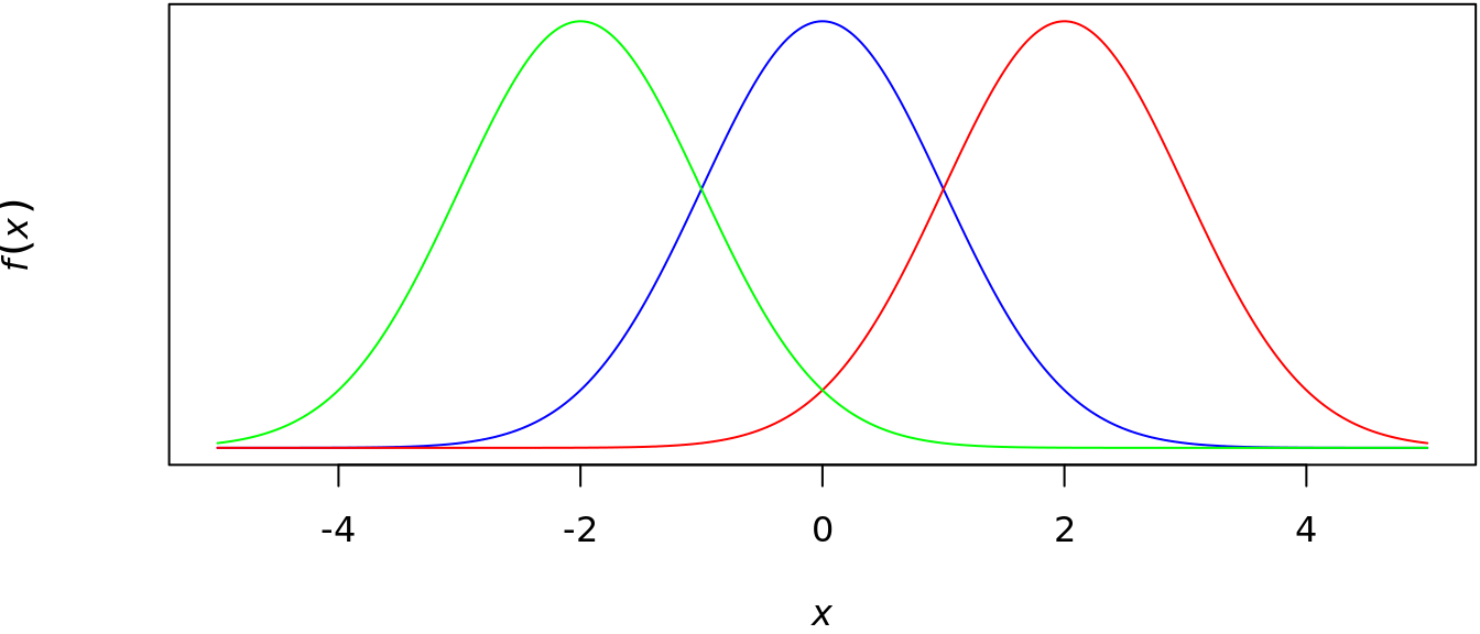
Figure 5.1: example of a normal location family

5.2.2 Scale families

Definition 5.4 Let \(f\left(x\right)\) be any pdf. Then, for any \(\sigma>0\), the family of pdfs \(\left(1/\sigma\right)f\left(x/\sigma\right)\), indexed by the parameter \(\sigma\), is called the scale family with standard pdf \(f\left(x\right)\) and \(\sigma\) is called the scale parameter of the family.

For example, \(f\left(x\right)\sim\mathcal{N}\left(0,1^{2}\right)\), \(\mathcal{N}\left(0,\sigma^{2}\right)\) is a scale family. The effect of introducing the scale parameter \(\sigma\) is either to stretch (\(\sigma>1\)) or to contract (\(\sigma<1\)) the graph of \(f\left(x\right)\) while still maintaining the same basic shape of the graph. Figure 5.2 shows the normal distribution with \(\mu=0\) and \(\sigma^{2}\in\left\{0.75^{2},1^{2},1.5^{2}\right\}=1^{2}\) green, red, and blue, respectively.

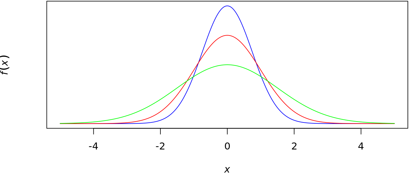
Figure 5.2: example of a normal scale family

Theorem 5.4 Let \(f\left(x\right)\) be any pdf. Let \(\mu\) be any real number, and let \(\sigma\) be any positive real number. Then \(X\) is a random variable with pdf \(\left(1/\sigma\right)f\left(\left(x-\mu\right)/\sigma\right)\) if and only if there exists a random variable \(Z\) with pdf \(f\left(z\right)\) and \(X=\sigma Z+\mu\).

(This is Theorem 3.5.6 from Casella and Berger (2002); the following proof is based on one given there.)

Proof. To prove the “if” part, define \(g\left(z\right)=\sigma z+\mu\), so that

\[ X=g\left(Z\right)=\sigma Z +\mu\implies Z=\frac{X-\mu}{\sigma}. \]

We have

\[ g^{-1}\left(x\right) = g^{-1}\left(g\left(z\right)\right) = z = \frac{x-\mu}{\sigma} \]

and

\[ \left|\frac{\dif}{\dif x}g^{-1}\left(x\right)\right|=\left|\frac{1}{\sigma}\right|=\frac{1}{\sigma}, \]

which is continuous on \(\mathbb{R}\). Noting that \(g\) is monotone, Theorem 3.5 implies that the pdf of \(X\) is

\[ f_{X}\left(x\right) = f_{Z}\left(g^{-1}\left(x\right)\right)\left|\frac{\dif}{\dif x}g^{-1}\left(x\right)\right| = f_{Z}\left(z\right)\frac{1}{\sigma} = \frac{1}{\sigma}f\left(\frac{x-\mu}{\sigma}\right). \]

To prove the “only if” part, define \(g\left(x\right)=\left(x-\mu\right)/\sigma\), and let

\[ Z=g\left(X\right)=\frac{X-\mu}{\sigma}\implies X=\sigma Z+\mu. \]

We have

\[ g^{-1}\left(z\right)=g^{-1}\left(g\left(x\right)\right) = x = \sigma z+\mu \]

and

\[ \left|\frac{\dif}{\dif z}g^{-1}\left(z\right)\right|=\left|\sigma\right|=\sigma, \]

which is continuous on \(\mathbb{R}\). Noting that \(g\) is monotone, Theorem 3.5 implies that the pdf of \(Z\) is

\[ f_{Z}\left(z\right) = f_{X}\left(g^{-1}\left(z\right)\right)\left|\frac{\dif}{\dif z}g^{-1}\left(z\right)\right| = f_{X}\left(x\right)\sigma = \frac{1}{\sigma}f\left(\frac{x-\mu}{\sigma}\right)\sigma = f\left(z\right). \]

Theorem 5.5 Let \(Z\) be a random variable with pdf \(f\left(z\right).\) Suppose \(\E\left[Z\right]\) and \(\Var\left(Z\right)\) exist. If \(X\) is a random variable with pdf \(\left(1/\sigma\right)f\left(\left(x-\mu\right)/\sigma\right)\), then

\[ \E\left[X\right]=\sigma\E\left[Z\right]+\mu\quad\text{and}\quad\Var\left(X\right)=\sigma^{2}\Var\left(Z\right). \]

(This is Theorem 3.5.7 from Casella and Berger (2002).)

Proof.

By Theorem 5.4, there is a random variable \(Z^{\ast}\) with pdf \(f\left(z\right)\) and \(X=\sigma Z^{\ast}+\mu\). So

\[ \begin{align*} \E\left[X\right] & =\E\left[\sigma Z^{\ast}+\mu\right] \\ & = \sigma\E\left[Z^{\ast}\right]+\mu \\ & = \sigma\int z^{\ast}\cdot f\left(z^{\ast}\right)\dif z^{\ast}+\mu \\ & = \sigma\int z\cdot f\left(z\right)\dif z+\mu \\ & =\sigma\E\left[Z\right]+\mu, \end{align*} \]

where the penultimate equality follows because \(Z^{\ast}\) has the same pdf as \(Z\). Next,

\[ \begin{align*} \Var\left(X\right) & = \E\left[\left(X-\E\left[X\right]\right)^{2}\right] \\ & = \E\left[\left(\sigma Z^{\ast}+\mu-\E\left[\sigma Z^{\ast}+\mu\right]\right)^{2}\right] \\ & = \E\left[\left(\sigma Z^{\ast}+\mu-\left(\sigma\E\left[Z^{\ast}\right]+\mu\right)\right)^{2}\right] \\ & = \E\left[\left(\sigma\left(Z^{\ast}-\E\left[Z^{\ast}\right]\right)\right)^{2}\right] \\ & = \E\left[\sigma^{2}\left(Z^{\ast}-\E\left[Z^{\ast}\right]\right)^{2}\right] \\ & = \sigma^{2}\E\left[\left(Z^{\ast}-\E\left[Z^{\ast}\right]\right)^{2}\right] \\ & = \sigma^{2}\Var\left(Z^{\ast}\right) \\ & = \sigma^{2}\Var\left(Z\right), \end{align*} \]

where the final equality follows because \(Z^{\ast}\) has the same pdf as \(Z\), and the result has been shown.

References

Casella, G., and R.L. Berger. 2002. Statistical Inference. Duxbury Advanced Series in Statistics and Decision Sciences. Thomson Learning. https://books.google.com/books?id=0x\_vAAAAMAAJ.