Chapter 11 PageRank
11.1 Motivation
Imagine a web surfer who moves from page to page by clicking on links randomly with uniform probability. Suppose that the surfer is confined to a set of five pages defined by the following graph, where a link from page \(i\) to page \(j\) is represented by an arrow pointing from \(i\) to \(j\).
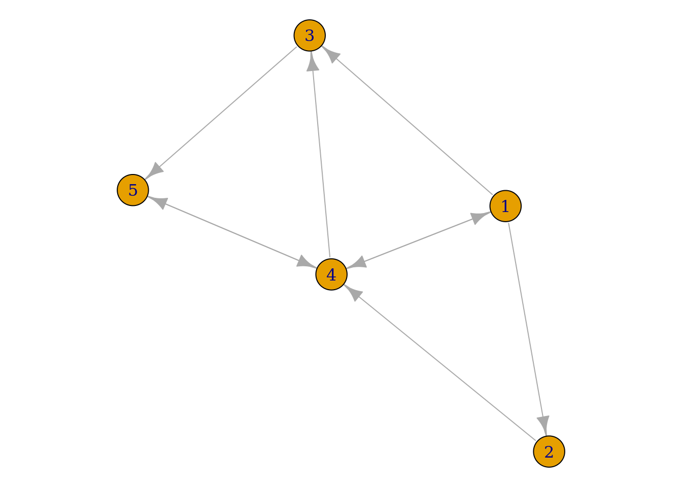
If the surfer is currently on page \(i\), we can represent the probability that the surfer moves to page \(j\) by the \(\left(i,j\right)\text{th}\) entry of the following transition probability matrix:
\[ \mathbf{A}= \begin{bmatrix} 0 & \frac{1}{3} & \frac{1}{3} & \frac{1}{3} & 0\\ 0 & 0 & 0 & 1 & 0\\ 0 & 0 & 0 & 0 & 1\\ \frac{1}{3} & 0 & \frac{1}{3} & 0 & \frac{1}{3}\\ 0 & 0 & 0 & 1 & 0 \end{bmatrix} \]
Proposition 11.1 Let \(\mathbf{A}\) be a transition probability matrix as above.
- Let \(\boldsymbol{\lambda}\in\mathbb{R}^{n}\) be the eigenvalues of \(\mathbf{A}^{\mathsf{T}}\). Then, \(\max_{i\in\left\{1,\ldots,n\right\}}\left |\lambda_{i}\right |=1\).
- Let \(\mathbf{v}\) be the eigenvector with eigenvalue 1. Then, \(v_{i}\geq 0\).
- If a web surfer surfs for a long time, then \(P\left(\text{surfer ends on page }i\right)=v_{i}\), assuming \(\sum_{i}v_{i}=1\).
In Google’s PageRank algorithm, described in Page et al. (1999), the page rank is determined by the values of \(v_{i}\) in decreasing order.
To obtain a page’s rank, we must compute the dominant eigenvector and eigenvalue.
11.2 Computing eigenpairs
We now consider the problem of computing eigenvalues and eigenvectors. Recall that a scalar \(\lambda\) is an eigenvalue of an \(n\times n\) matrix \(\mathbf{A}\) if and only if it satisfies the characteristic equation \(\det\left(\mathbf{A}-\lambda\mathbf{I}_{n}\right)=0\), where \(\mathbf{I}_{n}\) is the \(n\)-dimensional identity matrix and \(\det\left(\mathbf{M}\right)\) is the determinant of \(\mathbf{M}\). If the characteristic equation is a polynomial of degree 4 or less, then an explicit algebraic solution may be obtained. If the characteristic equation is of degree 5 or higher, than an algebraic solution is impossible, and the eigenvalues must be approximted by numerical methods.
In general, the computational complexity of computing the eigenvectors of a (square) \(n\)-dimensional matrix, e.g., by the QR algorithm, is \(O\left(n^{3}\right)\), i.e., cubic in the dimension of the matrix. It is clear that for a network of even modest size, e.g., \(10^{5}\), this problem will not be tractable. If we reduce the problem to computing the dominant eigenvector rather than all eigenvectors, then we can use a more efficient algorithm.
11.3 Algorithm
We now present power iteration. Let \(\mathbf{A}\) be an \(n\times n\) matrix.
- Choose \(\mathbf{v}^{\left(0\right)}\in\mathbb{R}^{n}\) such that \(\mathbf{v}^{\left(0\right)}\neq\mathbf{0}\), and choose \(\epsilon>0\).
While \(\left\Vert \mathbf{v}^{\left(i\right)}-\mathbf{v}^{\left(i-1\right)}\right\Vert \geq \epsilon\)
- \(\mathbf{v}^{\left(i\right)}\gets\mathbf{A}\mathbf{v}^{\left(i-1\right)}\)
- \(\mathbf{v}^{\left(i\right)}\gets\mathbf{v}^{\left(i\right)}/\sum_{j}v_{j}^{\left(i\right)}\)
When the algorithm terminates, \(\mathbf{v}^{\left(i\right)}\) will be (approximately) the dominant eigenvector of \(\mathbf{A}\). We can then compute the dominant eigenvalue \(\lambda_{\max}\) by the Rayleigh quotient, i.e.,
\[ \lambda_{\max}=\dfrac{\left(\mathbf{v}^{\left(i\right)}\right)^{\mathsf{T}}\mathbf{A}\mathbf{v}^{\left(i\right)}}{\left\Vert \mathbf{v}^{\left(i\right)}\right\Vert_{2}^{2}}. \]
Proof. We now present a proof sketch for power iteration.
Let \(\left\{\lambda_{i}\right\}_{i=1}^{n}\) be the eigenvalues of \(\mathbf{A}\) such that \(\left|\lambda_{1}\right|>\left|\lambda_{2}\right|>\cdots>\left|\lambda_{n}\right|\), and let \(\left\{\mathbf{w}^{\left(i\right)}\right\}_{i=1}^{n}\) be the corresponding eigenvectors.
Suppose that the \(\mathbf{w}^{\left(i\right)}\) form a basis for \(\mathbb{R}^{n}\), and suppose that we begin power iteration with some \(\mathbf{v}^{\left(0\right)}\in\mathbb{R}^{n}\). Because the \(\mathbf{w}^{\left(i\right)}\) span \(\mathbb{R}^{n}\), we can express \(\mathbf{v}^{\left(0\right)}\) as a linear combination of the \(\mathbf{w}^{\left(i\right)}\), i.e.,
\[ \mathbf{v}^{\left(0\right)}=\sum_{i=1}^{n}c_{i}\mathbf{w}^{\left(i\right)} \]
where \(\left\{c_{i}\right\}_{i=1}^{n}\in\mathbb{R}^{n}\). At the first iteration of the algorithm, we left-multiply \(\mathbf{v}^{\left(0\right)}\) by \(\mathbf{A}\), which we can write as
\[ \mathbf{v}^{\left(1\right)}= \mathbf{A}\mathbf{v}^{\left(0\right)}= \sum_{i=1}^{n}c_{i}\mathbf{A}\mathbf{w}^{\left(i\right)}= \sum_{i=1}^{n}c_{i}\lambda_{i}\mathbf{w}^{\left(i\right)} \]
where the final equality follows because \(\mathbf{w}^{\left(i\right)}\) is an eigenvector of \(\mathbf{A}\). Observe that if \(\mathbf{v}\) is an eigenvector of \(\mathbf{A}\), then \(c\mathbf{v}\) is also an eigenvector of \(\mathbf{A}\) for some \(c\in\mathbb{R}\). We have \(c=\sum_{j}v_{j}^{\left(i\right)}\), so without loss of generality we will omit the normalization step of the algorithm.
At the second iteration, we left-multiply \(\mathbf{v}^{\left(1\right)}\) by \(\mathbf{A}\), which we can write as
\[ \mathbf{v}^{\left(2\right)}= \mathbf{A}\mathbf{v}^{\left(1\right)}= \mathbf{A}\mathbf{A}\mathbf{v}^{\left(0\right)}= \mathbf{A}^{2}\mathbf{v}^{\left(0\right)}= \sum_{i=1}^{n}c_{i}\lambda_{i}\mathbf{A}\mathbf{w}^{\left(i\right)}= \sum_{i=1}^{n}c_{i}\lambda_{i}^{2}\mathbf{w}^{\left(i\right)}. \]
We can see that \(\mathbf{v}^{\left(M\right)}\) will have the form
\[ \mathbf{v}^{\left(M\right)}= \mathbf{A}^{M}\mathbf{v}^{\left(0\right)}= \sum_{i=1}^{n}c_{i}\lambda_{i}^{M}\mathbf{w}^{\left(i\right)}= c_{1}\lambda_{1}^{M}\mathbf{w}^{\left(1\right)}+ c_{2}\lambda_{2}^{M}\mathbf{w}^{\left(2\right)}+\cdots+ c_{n}\lambda_{n}^{M}\mathbf{w}^{\left(n\right)}. \]
We can factor out \(\lambda_{1}^{M}\) to give
\[ \mathbf{v}^{\left(M\right)}= \lambda_{1}^{M}\left( c_{1}\mathbf{w}^{\left(1\right)}+ c_{2}\left(\dfrac{\lambda_{2}}{\lambda_{1}}\right)^{M}\mathbf{w}^{\left(2\right)}+\cdots+ c_{n}\left(\dfrac{\lambda_{n}}{\lambda_{1}}\right)^{M}\mathbf{w}^{\left(n\right)} \right) \]
By assumption, \(\lambda_{1}\) is the largest eigenvalue of \(\mathbf{A}\), so that
\[ \left|\dfrac{\lambda_{i}}{\lambda_{1}}\right|<1,\quad i\in\left\{2,\ldots,n\right\}. \]
Thus,
\[ M\rightarrow\infty\implies\left(\dfrac{\lambda_{i}}{\lambda_{1}}\right)^{M}\rightarrow 0, \]
so that for some large but finite \(M\),
\[ \mathbf{v}^{\left(M\right)}\approx \lambda_{1}^{M}\left( c_{1}\mathbf{w}^{\left(1\right)}+ c_{2}\cdot 0\cdot\mathbf{w}^{\left(2\right)}+\cdots+ c_{n}\cdot 0\cdot\mathbf{w}^{\left(n\right)} \right)= \lambda_{1}^{M}c_{1}\mathbf{w}^{\left(1\right)}. \]
Let \(\tilde{\mathbf{w}}^{\left(1\right)}=\lambda_{1}^{M}c_{1}\mathbf{w}^{\left(1\right)}\), so that \(\mathbf{v}^{\left(M\right)}\approx\tilde{\mathbf{w}}^{\left(1\right)}\). The final step of the algorithm is to normalize \(\mathbf{v}^{\left(M\right)}\), i.e.,
\[ \mathbf{v}^{\left(M\right)}\approx \dfrac{\tilde{\mathbf{w}}^{\left(1\right)}}{\sum_{j}\tilde{w}_{j}^{\left(1\right)}}. \]
Thus, we see that \(\mathbf{v}^{\left(M\right)}\) approximates the dominant eigenvector \(\mathbf{w}^{\left(1\right)}\) of \(\mathbf{A}\), completing the proof sketch.11.4 Considerations
11.4.1 Connection to Markov chains
We can model the web surfer’s behavior by a Markov chain with transition probability matrix \(\mathbf{A}\). Suppose that \(\boldsymbol{\pi}\) is the stationary distribution of the chain, so that
\[ \boldsymbol{\pi}^{\mathsf{T}}\mathbf{A}=\boldsymbol{\pi}^\mathsf{T}\implies \mathbf{A}^\mathsf{T}\boldsymbol{\pi}=\boldsymbol{\pi}. \]
We can thus view power iteration as finding the stationary distribution of the Markov chain, the \(j\text{th}\) element of which can be interpreted as the long-run proportion of time the chain spends in state \(j\). Observe also that power iteration normalizes \(\mathbf{v}^{\left(i\right)}\) such that its components sum to 1, as required for a probability distribution.
11.4.2 Calculating the dominant eigenvalue
We stated above that we can find the eigenvalue corresponding to \(\mathbf{w}^{\left(1\right)}\) by the Rayleigh quotient. We have
\[ \dfrac{\left(\mathbf{w}^{\left(1\right)}\right)^{\mathsf{T}}\mathbf{A}\mathbf{w}^{\left(1\right)}}{\left\Vert\mathbf{w}^{\left(1\right)}\right\Vert_{2}^{2}}= \dfrac{\lambda_{1}\left(\mathbf{w}^{\left(1\right)}\right)^{\mathsf{T}}\mathbf{w}^{\left(1\right)}}{\left\Vert\mathbf{w}^{\left(1\right)}\right\Vert_{2}^{2}}= \lambda_{1}\dfrac{\left\Vert\mathbf{w}^{\left(1\right)}\right\Vert_{2}^{2}}{\left\Vert\mathbf{w}^{\left(1\right)}\right\Vert_{2}^{2}}= \lambda_{1}, \]
as desired.
11.4.3 Computational complexity
At each step of power iteration, we must compute \(\mathbf{A}\mathbf{v}^{\left(i-1\right)}\). The first entry of this product is obtained by summing the product of the first row of \(\mathbf{A}\) with \(\mathbf{v}^{\left(i-1\right)}\), which requires \(n\) multiplications. We have \(\mathbf{A}\sim n\times n\), i.e., we must repeat this process \(n\) times, so that computing \(\mathbf{A}\mathbf{v}^{\left(i-1\right)}\) requires \(n^{2}\) multiplications.
Thus, each step of power iteration has \(O\left(n^{2}\right)\) complexity. While this is an improvement over cubic complexity, it is still intractable for real-world problems, e.g., if we assume that the Internet has on the order of one billion web pages, i.e., \(n=10^{9}\), then power iteration requires \(10^{18}\) multiplications at each step. If we suppose that a typical laptop computer can execute on the order of one billion operations per second, then one step of power iteration on the Internet would require \(10^{18}/10^{9}=10^{9}\) seconds, or roughly 32 years (to say nothing of the memory requirements).
Observe that the quadratic complexity of a step of power iteration arises from our assumption that each component of \(\mathbf{A}\mathbf{v}^{\left(i-1\right)}\) must be computed. If we knew in advance the result of certain of these multiplications, we might not have to perform them. In particular, if we knew that the \(\left(i,j\right)\text{th}\) entry of \(\mathbf{A}\) were zero, then we would also immediately know that the \(j\text{th}\) summand in the product of the \(i\text{th}\) row of \(\mathbf{A}\) and \(\mathbf{v}^{\left(i-1\right)}\) is zero, and we could avoid doing that multiplication.
Sparse matrices enable precisely this kind of savings: they represent matrices in such a way as to avoid multiplications by zero. It remains to consider the characteristics of the network of interest, so that we might determine whether a sparse representation would be advantageous. Suppose that each web page links to on the order of 10 other pages. In this case, only 10 entries of each row of \(\mathbf{A}\) are nonzero, and the remaining \(10^{9}-10\) entries are zero. We must perform just 10 multiplications per row, and \(\mathbf{A}\) has \(10^{9}\) rows, so that a single step of power iteration requires just \(10^{10}\) multiplications, or roughly 10 seconds at \(10^{9}\) operations per second.
11.4.4 Convergence
The approximation \(\mathbf{v}^{\left(M\right)}\approx\mathbf{w}^{\left(1\right)}\) depends on the terms involving the other eigenvectors \(\left\{\mathbf{w}^{\left(i\right)}\right\}_{i=2}^{n}\) shrinking toward the zero vector. The rate at which the \(i\text{th}\) term converges to the zero vector is given by the ratio of \(\lambda_{i}\) to \(\lambda_{1}\). We assume that the eigenvalues are ordered by absolute value, hence the largest such term is \(\lambda_{2}/\lambda_{1}\), and this term will determine the rate of convergence of power iteration, e.g., if this ratio is close to 1, then the algorithm may converge slowly.
For large matrices, \(\lambda_{2}/\lambda_{1}\) will be close to 1. Google dealt with the slow convergence by modifying the web surfer model. First, choose \(p\in\left[0,1\right]\) (Google originally chose \(p\approx0.15\)). Then, assume that with probability \(p\) the web surfer randomly, with uniform probability, jumps to any page in the network given in \(\mathbf{A}\) and with probability \(\left(1-p\right)\) the surfer randomly, with uniform probability, jumps to a page with a link given in the current page. Thus, rather than surfing behavior governed exclusively by the probability transition matrix, the surfer may also make a random jump to any page in the network. We can represent this new behavior by replacing \(\mathbf{A}\) by
\[ \mathbf{M}=\left(1-p\right)\mathbf{A}+p\mathbf{B}, \]
where \(\mathbf{B}\) is a matrix with all entries given by \(1/n\), which \(n\) is again the number of pages in the network. Observe that if \(p=0\) this is equivalent to the original model.
The surfer’s behavior under this model can similarly be modeled by a Markov chain whose stationary distribution \(\mathbf{v}\) satisfies \(\mathbf{M}^{\mathsf{T}}\mathbf{v}=\mathbf{v}\). We can again approximate the stationary distribution by power iteration. We must be careful in implementation because while \(\mathbf{A}\) is typically sparse, \(\mathbf{M}\) never is (\(\mathbf{B}\) has all non-zero entries). It turns out that we can decompose \(\mathbf{M}^{\mathsf{T}}\mathbf{v}\) as
\[ \mathbf{M}^{\mathsf{T}}\mathbf{v}= \left(1-p\right)\mathbf{A}^{\mathsf{T}}\mathbf{v}+\dfrac{p}{n}\mathbf{1}\sum_{i=1}^{n}v_{i}, \]
where \(\mathbf{1}\) is the \(n\)-dimensional vector of ones. This decomposition allows us to compute the dominant eigenvector of the sparse matrix \(\mathbf{A}^\mathsf{T}\) rather than the dense matrix \(\left(\left(1-p\right)\mathbf{A}+p\mathbf{B}\right)^{\mathsf{T}}\), with the accompanying decrease in computational complexity. We now implement power iteration for this model.
#' Modified power iteration
#'
#' @param A adjacency matrix of original network
#' @param v0 starting vector
#' @param p probability of jumping to any page in `A`
#' @param tol iteration tolerance
#' @param niter maximum number of iterations
#'
#' @return list containing the number of iterations to converge and the
#'  dominant eigenvector of `A`
power_iter <- function(A, v0, p, tol = 1e-4, niter = 1e3) {
  mag <- function(x) sqrt(sum(x ^ 2))

  # normalize v0 so that convergence can occur in a single iteration
  v_old <- v0 / sum(v0)

  i <- 0
  delta <- tol + 1

  # this term does not change from iteration to iteration
  u <- (p / length(v0)) * rep(1, length(v0))

  while (i < niter && delta > tol) {
    v_new <- (1 - p) * crossprod(A, v_old) + sum(v_old) * u
    v_new <- v_new / sum(v_new)
    delta <- mag(v_new - v_old)
    v_old <- v_new
    i <- i + 1
  }
  list(
    niter = i,
    v = as.vector(v_new)
  )
}
We will test our implementation using the General Relativity network from the Stanford Network Analysis Project.
path <- "data/ca-GrQc.txt.gz"
if (!fs::file_exists(path)) {
  download.file(
    "http://snap.stanford.edu/data/ca-GrQc.txt.gz",
    destfile = path,
    quiet = TRUE
  )
}
gr <- readr::read_tsv(path, skip = 4, col_names = c("from", "to"))
gr
## # A tibble: 28,980 x 2
## from to
## <dbl> <dbl>
## 1 3466 937
## 2 3466 5233
## 3 3466 8579
## 4 3466 10310
## 5 3466 15931
## 6 3466 17038
## 7 3466 18720
## 8 3466 19607
## 9 10310 1854
## 10 10310 3466
## # … with 28,970 more rowsWe now implement a function to perform power iteration, measure its runtime, and extract the name of the top node, i.e., \(v_{\max}=\max_{j\in\left\{1,\ldots,n\right\}}v_{j}\).
#' Power iteration runtime and top node
#'
#' @param A adjacency matrix for power iteration
#' @param p probability of jumping to any page in `A`
#' @param ... other arguments passed to `power_iter()`
#'
#' @return list containing `p`, the name of the top node, the number of
#'   iterations required to converge, and the runtime
top_node <- function(A, p, ...) {
  runtime <- system.time(
    pi_result <- power_iter(
      A = A,
      v0 = rep(1, nrow(A)),
      p = p,
      ...
    )
  )
  # extract the (first) top-rated node
  v_max <- (rownames(A))[which.max(pi_result$v)]
  list(
    p = p,
    top_node = v_max,
    niter = pi_result$niter,
    time = runtime["elapsed"]
  )
}
Finally, we implement a function to perform power iteration for multiple values of \(p\). Note that gr is an edgelist.
#' Power iteration for multiple jump probabilities with sparse matrices
#'
#' @param el data frame containing a symbolic edge list in the first two
#'  columns; passed to `igraph::graph_from_data_frame()`
#' @param p vector of probabilities
#' @param sparse whether to use sparse matrices
#'
#' @return a tibble containing a row for each value of `p`, the name of the
#'  top node, the number of iterations required to converge, and the runtime
pagerank <- function(el, p, sparse = TRUE) {
  graph <- igraph::graph_from_data_frame(el)
  adj <- igraph::as_adjacency_matrix(graph, sparse = sparse)
  purrr::map_dfr(p, top_node, A = adj)
}
We are now ready to examine the impact of \(p\).
prob <- c(10 ^ -(6:2), 0.15, 0.5, 0.9, 0.99)
pr_dense <- pagerank(gr, p = prob, sparse = FALSE)
pr_dense
## # A tibble: 9 x 4
## p top_node niter time
## <dbl> <chr> <dbl> <dbl>
## 1 0.000001 21012 31 1.86
## 2 0.00001 21012 31 1.79
## 3 0.0001 21012 31 1.77
## 4 0.001 21012 31 1.79
## 5 0.01 21012 31 1.81
## 6 0.15 21012 31 1.79
## 7 0.5 21012 31 1.99
## 8 0.9 21012 30 1.74
## 9 0.99 21012 4 0.223We see that the top-rated node is 21012, and that 31 iterations were required for most values of \(p\). As \(p\) becomes large, the number of iterations required to converge decreases. We now repeat the process with sparse matrices.
pr_sparse <- pagerank(gr, p = prob)
pr_sparse
## # A tibble: 9 x 4
## p top_node niter time
## <dbl> <chr> <dbl> <dbl>
## 1 0.000001 21012 31 0.059
## 2 0.00001 21012 31 0.0460
## 3 0.0001 21012 31 0.0460
## 4 0.001 21012 31 0.0460
## 5 0.01 21012 31 0.048
## 6 0.15 21012 31 0.046
## 7 0.5 21012 31 0.0460
## 8 0.9 21012 30 0.0440
## 9 0.99 21012 4 0.006We see that the same number of iterations are required to converge as in the dense case, but that the time required is decreased by roughly two orders of magnitude. Finally, observe that node 21012 is also the node with the largest number of adjacent vertices (connections) (note that the ego graph of a vertex includes the vertex itself):
graph <- igraph::graph_from_data_frame(gr)
igraph::neighbors(graph, v = "21012")
## + 81/5242 vertices, named, from 847be67:
## [1] 10243 6610 22691 2980 18866 25758 11241 13597 3409 15538 570
## [12] 8503 18719 9889 773 9341 21847 6179 1997 2741 13060 14807
## [23] 24955 45 4511 21281 23293 9482 15003 20635 22457 19423 5134
## [34] 3372 23452 23628 2404 22421 18894 18208 1234 25053 18543 4164
## [45] 7956 12365 17655 25346 1653 9785 21508 14540 12781 1186 345
## [56] 2212 231 46 19961 2952 6830 8879 11472 12496 12851 15659
## [67] 17692 20108 20562 22887 6774 4513 25251 12503 22937 23363 5578
## [78] 1841 16611 2450 8049graph %>% igraph::ego_size() %>% max()## [1] 82Finally, observe that PageRank is a variant of eigenvector centrality:
ec <- igraph::eigen_centrality(graph)
ec$vector[which.max(ec$vector)]
## 21012
## 1In eigenvector centrality, the score of a node is increased more by (inbound) connections from high-scoring nodes than from low-scoring nodes. There are several other important types of centrality, e.g., betweenness centrality, in which the score of a node is determined by how often it appears in the shortest path between two other nodes (how often it acts as a “bridge”).
References
Page, Lawrence, Sergey Brin, Rajeev Motwani, and Terry Winograd. 1999. “The Pagerank Citation Ranking: Bringing Order to the Web.” Technical Report 1999-66. Stanford InfoLab; Stanford InfoLab. http://ilpubs.stanford.edu:8090/422/.